Robotic Planning and Kinematics

1. Sensor-Based Motion Planning

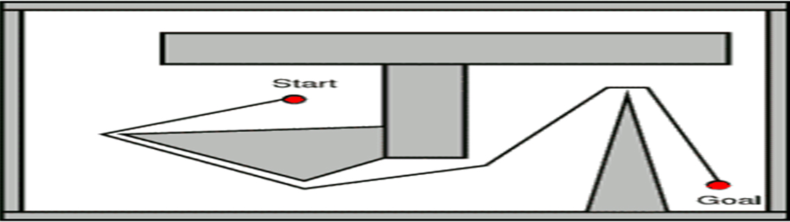
Motion planning is an important and common problem in robotics. In its simplest form, the motion planning problem is: how to move a robot from a “start” location to a “goal” location avoiding obstacles.

Robot Assumptions

knows the direction towards the goal,
knows the straight-line distance between itself and the goal,
does not know anything about the obstacles (number, location, shape, etc.)
has a contact sensor that allows it to locally detect obstacles,
can move either in a straight line towards the goal or can follow an obstacle boundary (possibly by using its contact sensor), and
has limited memory in which it can store distances and angles.

Environment Assumptions

the workspace is bounded
there are only a finite number of obstacles
the start and goal points are in the free workspace
any straight line drawn in the environment crosses the boundary of each obstacle only a finite number of times. (This assumption is easily satisfied for “normal objects”.)

Compute Line Through Two Points
Input: two distinct points P1 = (x1,y1) and P2 = (x2,y2) on the plane
Output: parameters (a,b,c) defining the line {(x,y) | ax + by + c = 0} that passes through both P1 and P2. Normalize the parameters so that a² + b² = 1.

Using Matlab

function [a,b,c] = line_points(p1,p2)
A = [p1(1,1) p2(1,1)];
B = [p1(1,2) p2(1,2)];
if (p1(1,1) == p2(1,1))
	a = 1;
	b = 0;
	c = -p1(1,1);
else
	p = polyfit(A,B,1);
	slope = p(1,1);
	intercept = p(1,2);
	a = slope/sqrt(slope^2 + 1);
	b = -sqrt(1 - a^2);
	c = intercept • -b;
	if c < 10^-10
		c = 0;
	end
end
disp(['ax + by + c = 0'])
end

Compute Distance Point To Line
Input: a point q and two distinct points P1 = (x1,y1) and P2 = (X2,Y2) defining a line.
Output: the distance from q to the line defined by P1 and P2.

Using Matlab

function [distance] = d_pl(p1,p2,Q)
%P1,P2,Q are written as [x,y] format
A = [p1(1,1) p1(1,2) 0];
B = [p1(1,1) p2(1,2)0];
Q = [Q(1,1) Q(1,2) 0];
AB = A - B;
BQ = Q - B;
ABBQ = cross(AB,BQ);
distance = norm(ABBQ)/norm(AB);
end

Compute Distance Point To Segment
Input: a point q and a segment defined by two distinct points (P1,P2).
Output: the distance from q to the segment with extreme points (P1,P2).

Using Matlab

function [distance] = d_ps(p1,p2,Q)
%P1,P2,Q are written as [x,y] format
A = [p1(1,1) p1(1,2)];
B = [p2(1,1) p2(1,2)];
Q = [Q(1,1) Q(1,2)];
AB = norm(A - B);
AQ = norm(A - Q);
BQ = norm(B - Q);
if dot(A - B, Q - B) • dot(Q - A, Q - A) >= 0
	x = [A,1;B,1;Q,1];
	distance = abs(det(x))/AB;
else
	distance = min(AQ,BQ);
end
end

Compute Distance Point To Polygon
Input: a polygon P and a point q.
Output: the distance from q to the closest point in P, called the distance from q to the polygon.

Using Matlab

function [distance] = d_pp(P,Q)
%P is written as [x1,y1;x2,y2;...] format and Q is written as [x,y] format
n = length(P);
i = 1;
d = [];
while i < n
	A = [P(i,1) P(i,2)];
	B = [P(i + 1,1) P(i + 1,2)];
	Q = [Q(1,1) Q(1,2)];
	AB = norm(A - B);
	AQ = norm(A - Q);
	BQ = norm(B - Q);
	if dot(A - B, Q - B) • dot(B - A, Q - A) >= 0
		X = [A,1;B,1;Q,1];
		x = sym(X);
		distance = abs(det(x))/AB;
	else
		distance = min(AQ,BQ);
	end
	d(1,i) = distance;
	i = i + 1:
end
A = [P(1,1) P(1,2)];
B = [P(n,1) P(n,2)];
Q = [Q(1,1) Q(1,2)];
AB = norm(A - B);
AQ = norm(A - Q);
BQ = norm(B - Q);
if dot(A - B,Q - B) • dot(B - A,Q - A) >= 0
	X = [A,1;B,1;Q,1];
	x = sym(X);
	distance = abs(det(x))/AB;
else
	distance = min(AQ,BQ);
end
d(1,n) = distance;
distance = min(d);
end

Compute tangent Vector To polygon
Input: a polygon P and a point q.
Output: the unit-length vector u tangent at point q to the polygon P in the following sense: (i) if q is closest to a segment of the polygon, then u should be parallel to the segment, (ii) if q is closest to a vertex, then u should be tangent to a circle centered at the vertex that passes through q, and (iii) the tangent should lie in the counter-clockwise direction.

Using Matlab

function [u] = v_pp(P,Q)
n = length(P);
i = 1;
d = [];
%Finding shortest dist from 1->n
while i < n
	A = [P(i,1) P(i,2)];
	B = [P(i+1,1) P(i+1,2)];
	Q = [Q(1,1) Q(1,2)];
	AB = norm(A - B);
	AQ = norm(A - Q);
	BQ = norm(B - Q);
	if dot(A - B, Q - B) • dot(B - A, Q - A) >= 0
		X = [A,1;B,1;Q,1];
		x = sym(X);
		distance - abs(det(x))/AB;
	else
		distance = min(AQ,BQ);
	end
	d(1,i) = distance;
	i = i + 1;
end
%Find dist from n->1
A = [P(1,1)	P(1,2)];
B = [P(n,1)	P(n,2)];
Q = [Q(1,1)	Q(1,2)];
AB = norm(A - B);
AQ = norm(A - Q);
BQ = norm(B - Q);
if dot(A - B,Q - B) • dot(B - A, Q - A) >= 0
	X = [A,1;B,1;Q,1];
	x = sym(X);
	distance = abs(det(x))/AB;
else
	distance = min(AQ,BQ);
end
d(1,n) = distance;
distance = min(d);
f = find(ismember(d,distance), 1);
if f == n;
	g = 1;
else
	g = f + 1;
end
x1 = P(f,1) - Q(1,1);
y1 = P(f,2) - Q(1,2);
x2 = P(g,1) - Q(1,1);
y2 = P(g,2) - Q(1,2);
c1 = sqrt(x1^2 + y1^2);
c2 = sqrt(x2^2 + y2^2);
l1 = sqrt((P(f,1) - P(g,1))^2 + (P(f,2) - P(g,2))^2);
if distance ~= c1 & distance ~= c2;
	l2 = sqrt(c2^2 - distance^2);
	xcenter = l2/l1 • (x1 - x2);
	ycenter = l2/l1 • (y1 - y2);
	center = [P(g,1) + xcenter,P(g, 2) + ycenter];
	x3 = center(1,1) - Q(1,1);
	y3 = center(1,2) - Q(1,2);
	u = [y3,-x3];
	u = u/distance;
elseif c1 < c2
	u = [y1,-x1];
	u = u/distance;
elseif c2 < c1
	u = [y2,-x2];
	u = u/distance;
end
%Check if length = 1
%u(1,1)^2 + u(1,2)^2
end

The Bug0 Algorithm

while not at goal:

   move towards the goal

   if hit an obstacle:

      while not able to move towards the goal:

         follow the obstacle’s boundary moving to the left

Unfortunately, Bug0 algorithm does not work properly in the sense that there are situations (workspace, obstacles, start and goal positions) for which there exists a solution (a path from start to goal) but the Bug0 algorithm does not find it.

The Bug1 Algorithm

while not at goal:

   move towards the goal

   if hit an obstacle:

      circumnavigate it(moving to the left or right is unimportant). While circumnavigating, store in memory the minimum distance from the obstacle boundary to the goal

      follow the boundary back to the boundary point with minimum distance to the goal

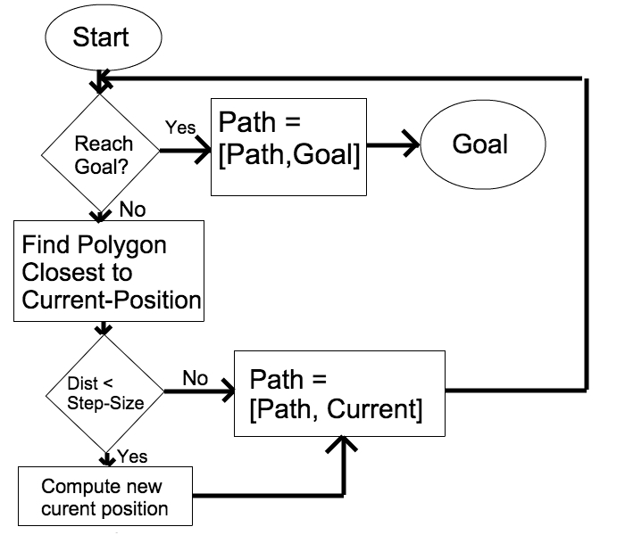
Flowcharts

Circles represent the start and terminating points
Arrows indicate the flow of control
Rectangles represent a single command
Diamonds output 2 paths based on binary question

Sketch a flowchart and implement the BugBase algorithm.
The BugBase Algorithm
Input: Two locations start and goal in W, a list of polygon obstacles obstaclesList, and a length step-size l.
Output: A sequence, denoted path, of points from start to the first obstacle between start and goal (or from start to goal if no obstacle lies between them). Successive points are separated by no more than step-size.

current-position = start

path = [start]

while distance(current-position,goal) > step-size:

   find polygon closest to current-position

   if distance from current-position to closest polygon < step-size:

      return “Failure: There is an obstacle lying between the start and goal” and path

      compute new current-position by taking a step of length step-size towards goal

      path = [path,current-position]

path = [path,goal]

return “Success” and path

Compute Bug1
Input: Two locations start and goal in W, a list of polygonal obstacles obstacleList, and a length step-size
Output: A sequence, denoted path, of points from start to goal or returns an error message if such a path does not exists. Successive points are separated by no more than step-size and are computed according to the Bug 1 algorithm.

Using Matlab

function [path] = Bug_One(S,G,O,Step)
%S = starting point, G = goal point, O = obstacles, Step = Step Size
t = 0;
%Check if solvable or not
i = 1;
l = length (O);
start = [];
goal = [];
while i < l;
	[st] = inpolygon(S(1,1),S(1,2),(O{1,i}(:,1)),(O{1,i}(:,2)));
	[go] = inpolygon(G(1,1),G(1,2),(O{1,i}(:,1)),(O{1,i}(:,2)));
	i = i + 1;
	start = [start,st];
	goal = [goal,go];
end
if sum(start) > 0;
	disp('Failure: Start Point in Polygon');
	path = Nan;
	return;
elseif sum(goal) > 0;
	disp('Failure: Goal Point in Polygon');
	path = Nan;
	return;
else
	%Implement Bug 1 Algorithm
	current = S;
	path = [S];
	total = [];
	while norm(G-current) > Step;
		%Find the Closest polygon to S
		j = 1;
		Sclosest = [];
		while j <= l;
			P = O{i,j};
			Q = S;
			[distance] = d_pp(P,Q);
			Sclosest = [Sclosest,distance];   %Matrix dist S to Polygons
			j = j + 1;
			t = t + 1;
		end
		%Find the Closest Polygon toG
		jj = 1;
		Gclosest = [];
		while jj <=l;
			P = O{1,jj};
			Q = G;
			[distance = d_pp(P,Q)];
			Gclosest = [Gclosest, distance];   %Matrix dist G to polygons
			jj = jj + 1;
			t = t + 1;
		end
		while sum(Sclosest) < 200;
			%Getting Phit
			temp = min(Sclosest);
			[row,col] = find(Sclosest = temp);
			spot = col;
			k = 1;
			Oalt = [O{1,spot}; O{1,spot}(1,:)];
			xbox = [];
			ybox = [];
			while k <= (length(Oalt));
				xbox = [xbox,Oalt(k,1)];
				ybox = [ybox,Oalt(k,2)];
				k = k + 1;
				t = t + 1;
			end
			[xi,yi] = polyxpoly([current(1,1) G(1,1)],[current(1,2) G(1,2)], xbox, ybox);
			Phit = [xi(1,1) yi(1,1)];
			path = [path; Phit];
			total = [total, norm(Phit-current)];
			current = Phit;
			%Getting Pleave
			k = ((Oalt(1,2)-Oalt(3,2))•(G(1,1)-Oalt(3,1))-(Oalt(1,1)-Oalt(3,1))•(G(1,2)-Oalt(3,2))/((Oalt(1,2)-Oalt(3,2))^2+(Oalt(1,1)-Oalt(3,1))^2);
			x4 = G(1,1) - k • (Oalt(1,2) - Oalt(3,2));
			y4 = G(1,2) + k • (Oalt(1,1) - Oalt(3,1));
			Pleave = [x4,y4];
			%Going around Polygon
			r = 1;
			Z = O{1,spot};
			Z = sortrows(Z,2);
			while r <= length(O{1,spot});
				path = [path,Z(r,:)];
				total = [total,norm(Z(r,:) - current)];
				current = Z(r,:);
				r = r + 1;
			end
			path = [path; Phit];
			total = [total, norm(Phit-current)];
			current = Phit;
			r = 1;
			Z = [Z;Pleave];
			Z = sortrows(Z,2);
			while r < length(Z);
				path = [path;Z(r,:)];
				total = [total,norm(Z(r,:) - current)];
				current = Z(r,:);
				r = r + 1;
				t = t + 1;
			end
			Sclosest(1,spot) = 101;
			Gclosest(1,spot) = 0;
			t = t + 1;
		end
		total = [total,norm(G - current)];
		path = [path;G];
		current = G;
		total = sum(total);
		t = t + 1;
	end
end
hold on
%axis ([0 10 0 10])
plot(path(:,1),path(:,2))
end

Testing Bug1 Algorithm:
start = (0,0) and goal = (5,3)
step-size = 0.1 obstacleList = {(1,2),(1,0),(3,0)}, {(2,3),(4,1),(5,2)}

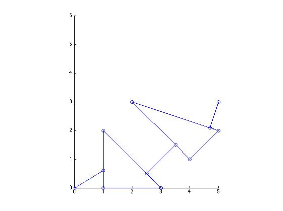
Path: (0,0)->(1,0.6)->(1,0)->(3,0)->(1,2)->(1,0.6)->(1,0)->(3,0)->(2.5,0.5)->(3.5,1.5)->(4,1)->(5,2)->(2,3)->(3.5,1.5)->(4,1)->(5,2)->(4.7,2.1)->(5,3)

Total Path Length: 23.5071

Time: 21

Bug2.prelim Algorithm

while not at goal:

   move towards the goal (along the start-goal-line)

   if hit an obstacle:

      follow the obstacle’s boundary (moving either left or right), until you encounter the start-goal-line again and are able to move towards the goal

This algorithm may cause the path to be longer than needed. For convenience we repeat the entire algorithm, but the only difference is the addition of the requirement that the leave point be closer to the goal than the hit point!

The Bug2 Algorithm

while not at goal:

   move towards the goal (along the start-goal-line)

   if hit an obstacle:

      follow the obstacle’s boundary (the turn direction is irrelevant), until you encounter the start-goal-line again closer to the goal and are able to move towards the goal

2. Motion Planning via Decomposition and Search

Robot Assumptions

knows the start and goal locations, and
knows the workspace and obstacles

World Assumptions

the workspace is a bounded polygon
there are only a finite number of obstacles that are polygons inside the workspace, and
the start and goal points are inside the workspace and outside all obstacles

The amount of time it takes for a motion planning algorithm to run, call it’s run-time rather than the length of the path it produces. The run-time of an algorithm is given by the number of computer steps required to execute the code.

Decomposition into convex subsets

For complex non-convex environments, we use an algorithm to decompose the free workspace into the union of convex subsets, such as triangles, convex quadrilaterals or trapezoids. The following nomenclature is convenient:
(i) the triangulation of the polygon is the decomposition of the polygon into a collection of triangles, and
(ii) the trapizoidation of the polygon is the decomposition of the polygon into a collective of trapezoids

The Sweeping Trapezoidation Algorithm

Input: a polygon possibly with polygonal holes
Output: a set of disjoint trapezoids, whose union equals the polygon

initialize an empty list T of trapezoids

order all vertices (of the obstacles and of the workspace) horizontally from left to right

for each vertex selected in a left-to-right sweeping order:

extend vertical segments upward and downwards from the vertex until they intersect an obstacle or the workspace boundary

add to T the new trapezoids, if any, generated by these segment(s)

Three key ideas we covered so far:
(1) convexity leads to very simple paths, (2) if the free workspace is not convex, it is easy to navigate between neighboring convex sets, (3) a complex free workspace can be decomposed into convex subsets via, for example, the sweeping trapezoidation algorithm.
The next observation is that the sweeping trapezoidation algorithm can easily be modified to additionally provide a list of neighborhood relationships between trapezoids.

The Roadmap-from-Decomposition Algorithm

Input: the trapezoidation of a polygon (possibly with holes)
Output: a roadmap

label the center of each trapezoid with the symbol ♢

label the midpoint of each vertical separating segment with the symbol ♦

for each trapezoid:

connect the center to all the midpoints in the trapezoid

return the roadmap consisting of centers, midpoints and their connections

The Planning-via-Decomposition + Search Algorithm

Input: free workspace W_free, start point p_start and goal point p_goal
Output: a path from p_start to p_goal if it exists, otherwise a failure notice. Either outcome is obtained in finite time.

compute a decomposition of W_free and the corresponding roadmap

in the decomposition, find the start trapezoid containing p_start and the goal trapezoid containing p_goal

in the roadmap, search for a path from start trapezoid to goal trapezoid

if no path exists from start trapezoid to goal trapezoid

   return failure notice

else

return path by concatenating:
      the segment from p_start to the center of start trapezoid
      the path from the start trapezoid to goal trapezoid
      the segment from the center of goal trapezoid to p_goal

The breadth-first search algorithm, also called BFS algorithm, is one of the simplest graph search strategy and is optimal in the sense that it computes shortest paths.

The breadth-first search (BFS) algorithm

Input: a graph G, a start node v_start and goal node v_goal
Output: a path from v_start to v_goal if it exists, otherwise a failure notice

create an empty queue Q and insert (Q,v_start)

for each node v in G:

   parent(v) = NONE

parent(v_start) = SELF

while Q is not empty:

   v = retrieve(Q)

   for each node u connected to v by an edge:

      if parent(u) == NONE:

         set parent(u) = v and insert (Q,u)

      if u == v_goal:

         run extract-path algorithm to compute the path from start to goal

         return success and the path from start to goal

return failure notice along with the parent pointers

The extract-path algorithm

Input: a goal node v_goal, and the parent pointers
Output: a path from v_start to v_goal

create an array P = [v_goal]

set u = v_goal

while parent(u) ≠ SELF:

u = parent(u)

insert u at the beginning of P

return P

computeBFStree
Input: a graph described by its adjacency table AdjTable, a start node start
Output: a vector of pointers parents describing the BFS tree rooted at start

Using Matlab

function [BFStree] = computeBFStree (AdjTable, start)
% Insert AdjTable as a [:,2] Matrix
s = AdjTable(:,1);
t = AdjTable(:,2);
l = length(AdjTable);
Q = [];
Q = [start,Q];
BFStree = [];
while isempty(Q) ~= 1
	pos1 = find(s == Q(1));
	pos2 = find(t == Q(1));
	adj1 = t(pos1);
	adj2 = s(pos2);
	adj = sort([adj1' adj2']);
	i = length(Q);
	j = length(BFStree);
	for n = 1:i
		del = find(adj == Q(n));
		adj(del) = [];
	end
	for m = 1:j
		del = find(adj == BFStree(m));
		adj(del) = [];
	end
	Q = [Q adj];
	if (Q(1) == BFStree) > 0
		Q(1) = [];
	else
		BFStree = [BFStree Q(1)];
		Q(1) = [];
	end
end
end

3. Configuration Spaces

describe a robot as a single or multiple interconnected rigid bodies,
define the configuration space of a robot,
examine numerous example configuration spaces,
discuss forward and inverse kinematic maps

Some simple concepts:
(i) a rigid body is a collection of particles whose position relative to one another is fixed,
(ii) a robot is composed of a single rigid body or multiple interconnected rigid bodies,
(iii) robots are 3-dimensional in nature, but we focus on plane problems for now.
(iv) it is equivalent to specify

Example Systems:

Disk robo- has the shape of a disk and is characterized by just one parameter, its radius r > 0. The disk robot does not have an orientation. Accordingly, the disk robots only motion is translation in the plane: that is, translations in the horizontal and vertical directions.
Translating polygon robot- has a polygonal shape. This robot is assumed to have a fixed orientation, and thus it’s only motion is translations in the plane.
Roto-translation polygon robot- has an arbitrary polygonal shape, is capable of translating in the horizontal and vertical directions as well as rotating.
Multi-link or multi-body robot- composed of multiple rigid bodies (or links) interconnected. Each link of the robot can rotate and translate in the plane, but these motions are constrained by connections to the other links and to the robot base.

Configuration Space

A configuration of a robot is a minimal set of variables that specifies the position and orientation of each rigid body composing the robot. The robot configuration is usually denoted bye the letter q
The configuration space is the set of all possible configurations of a robot. The robot configuration space is usually denoted by the letter Q, so that q ∈ Q.
The number of degrees of freedom of a robot is the dimension of the configuration space, i.e., the minimum number of variables required to fully specify the position and orientation of each rigid body belonging to the robot.
Given that the robot is at configuration q, we know where all points of the robot are.

4. Free Configuration Spaces via Sampling and Collision Detection

represent obstacles and the free space when the robot is composed of a single or multiple rigid bodies with proper shape, position and orientation
compute free configuration spaces via sampling and collision detection,
discuss sampling methods
discuss collision detection methods

Free configuration space for the disk robot

To compute the free configuration space and the obstacles in configuration space we reason as follows: a disk with radius r in collision with an obstacle if and only if the disk center is closer to the obstacle than r. Accordingly, we grow or “expand” the obstacle and, correspondingly, to “shrink” the workspace.
Using this key idea, the obstacle in configuration space is the expanded rectangle and the free configuration space of the disk robot is described in any of the two completely equivalent forms:

(i) the set of points of the disk center such that the disk does not intersect the obstacle and is inside the workspace,
(ii) the shrunk workspace minus the expanded obstacle.

Free configuration space for the translating polygonal robot

There is a simple graphical approach to computing the configuration space obstacle:

(i) move the robot to touch the obstacle boundary (recall the robot is not allowed to rotate),
(ii) slide the robot body along the obstacle boundary, maintaining the contact between the robot boundary and the obstacle boundary,
(iii) while sliding, store the location of the reference point of the robot: the resulting path encloses a convex polygon equal to the configuration space obstacle.

Sampling Methods

A sampling method should have certain properties:

Uniformity: the samples should provide a “good covering” of space. Mathematically, this can be formulated using the notion of dispersion
Incremental property: the sequence of samples should provide good coverage at any number n of samples. In other words, it should be possible to increase n continuously and not only in discrete large amounts.
Lattice structure: given a sample, the location of nearby samples should be computationally easy to determine.

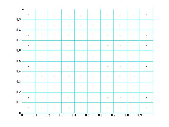
Uniform grids There are two ways of defining uniform grids in the unit cube. We call them the center grid and the corner grid. Both grids with n points can be defined if n = k^d for some number k.

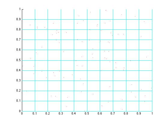
Random and pseudo-random sampling Adopting a random number generator is usually a very simple approach to (uniformly or possibly non-uniformly) sample the cube. Randomly-sampled points have asymptotically worse dispersion than center grids.

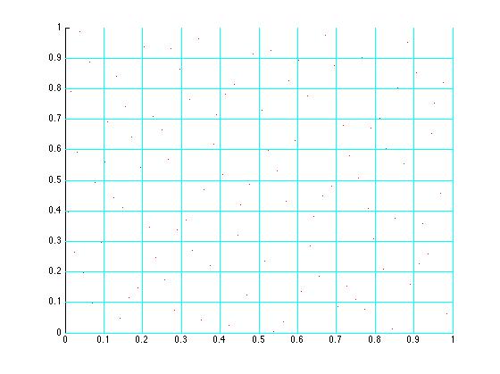
Halton sequences are an elegant way of sampling an interval with good uniformity (better than a pseudorandom sequence, though not as good as the optimal center grid) and with the incremental property (which the center grid does not posses).

The Halton sequence algorithm

Input: length of the sequence N ∈ N and prime number p ∈ N
Output: an array S[1…N] with the first N samples of the Halton sequence generated by p

initialize: S to be an array of N zeros

for each i from 1 to N:

   initialize: i_tmp = i, and f = 1/p

   while i_tmp > 0:

      compute the quotient q and the remainder r of the division i_tmp/p

      S(i) = S(i) + f • r

         i_tmp = q

      f = f/p

return S

Collision detection methods

The next step is to detect whether or not these configurations are in collision with an obstacle or workspace boundary. To do this we require several collision detection methods.

Basic primitive #1: is a point in a convex polygon?

Given a convex polygon with counter-clockwise vertices and a point q, the following conditions are equivalent:

(i) the point q is in the polygon (possibly on the boundary)
(ii) for all i ∈ {1,…,n}, the point q belongs to the halfplane with boundary line passing through the vertices p_i and p_i+1 and containing the polygon
(iii) for all i ∈ {i,…,n}, the dot product between the interior normal to the side p_ip_i+1 and the segment p_iq is positive or zero.
(Here the convention is that p_i+1 = p₁. A similar set of results can be given to check that the point is strictly inside the polygon.)

Basic primitive #2: do two segments intersect?

Any two lines in the plane are in one of three exclusive configurations: (1) parallel and coincident, (2) parallel and distinct, or (3) intersecting at a single point. In order for two segments to intersect, the two corresponding lines may be coincident (and the two segments need to intersect at least partly) or may intersect at a point (and the point must belong to the two segments). Now, if the two lines intersect at a point, one still needs to check that the intersection point actually belongs to the segment.

Basic primitive #3: do two convex polygons intersect?

There are five possible cases that one must consider, and each is illustrated below.

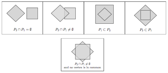
The convex-polygon-intersection algorithm

Input: two convex polygons P₁ and P₂
Output: collision or no collision

if (any vertex of P₁ belongs to P₂) OR (any vertex of P₂ belongs to P₁):

return collision

if any edge of P₁ intersects any edge of P₂:

return collision

return no collision

Given conditions:
Consider the unit square [0,1]² in the plane. Pick an arbitrary integer k and do:

write formulas for the n = k² sample points in the uniform Sukharev center grid;
write formulas for the n = k² sample points in the uniform corner grid;
write the following programs (representing a grid with n entries in [0,1]² by a matrix with n rows and 2 columns):

computeGridSukharev
Input: the number of samples n (assuming n = k² for some integer number k)
Output: the uniform Sukharev center grid on [0,1]² with [n^1/2] samples along each axis

Using Matlab

function [xpoints, ypoints] = GridSukharev(n)
k = sqrt(n);
if k ~= round(k);
	display 'Cannot Create Sukharev Grid';
	return;
end
%Change Parameters [0 1]^2 or [0 2*pi]^2
x = 0:2 • pi/k:2 • pi;
y = 0:2 • pi/k:2 • pi;
[xx,yy] = meshgrid(x,y);
xsize = size(xx);
ysize = size(yy);
i = 1;
xmid = [];
ymid = [];
temp = [];
while i < xsize(1,1);
	j = 1;
	while j < xsize(1,2);
		xmid = [xmid (xx(i,j+1)+xx(i,j))/2];
		j = j + 1;
	end
	temp = [xmid(1:(xsize-1)); temp];
	i = i + 1;
end
xmid = temp;
i = 1;
temp = [];
while i < ysize(1,2);
	j = 1;
	while j < ysize(1,1);
		ymid = [ymid (yy(j+1,i)+yy(j,i))/2];
		j = j + 1;
	end
	temp = [temp;ymid(1:(ysize - 1))];
	i = i + 1;
end
ymid = temp';
%Uncomment for plots
%hold on;
%axis equal;
%plot(xx,yy,'c');
%plot(xx',yy','c');
%plot(xmid,ymid,'r.')
xpoints = xmid;
ypoints = ymid;
end

Testing GridSukharev(100)

computeGridRandom
Input: the number of samples n
Output: the random grid on [0,1]² with n uniformly-generated samples

Using Matlab

function [xpoints,ypoints] = GridRandom(n)
k = sqrt(n);
r = randi(6,k,2);
x = r(:,1);
y = r(:,2);
if k != round(k);
	display 'Cannot Create Grid';
	return;
end
%Chagne Parameters [0 1]^2 or [0 2*pi]^2
xx = 0:2 • pi/k:2 • pi;
yy = 0:2 • pi/k:2 • pi;
[xxx,yyy] = meshgrid(xx,yy);
%hold on
%axis([0 1 0 1])
%plot(x,y,'r.');
%plot(xxx,yyy,'c');
%plot(xxx',yyy','c');
xpoints = x;
ypoints = y;
end

Testing GridRandom(100)

computeGridHalton
Input: the number of samples n; two prime numbers b₁ and b₂
Output: a Halton sequence of n samples inside [0,1]² generated by the prime numbers b₁ and b₂

Using Matlab

function [xpoints,ypoints] = GridHalton(n,b1,b2)
k = sqrt(n);
if k ~= round(k);
	display 'Cannot Create Grid';
	return;
end
S = zeros(1,n);
for i = 1:n;
	itemp = i;
	f = 1/b1;
	while itemp > 0;
		n1 = floor(itemp/b1);
		r = itemp - n1 • b1;
		S(i) = S(i) + f  r;
		f = f/b1;
		itemp = n1;
	end
end
T = zeros(1,n);
for i = 1:n;
	itemp = i;
	f = 1/b2
	while itemp > 0;
		n1 = floor(itemp/b2);
		r = itemp - n1 • b2;
T(i) = T(i) + f • r;
		f = f/b2;
		itemp = n1;
	end
end
xx = 0:1/k:1;
yy = 0:1/k:1;
[xxx,yyy] = meshgrid(xx,yy);
xsize = size(xxx);
ysize = size(yyy);
%hold on;
%axis([0 1 0 1]);
%plot(S,T,'r.');
%plot(xxx,yyy,'c');
%plot(xxx',yyy','c');
xpoints = S;
ypoints = T;
end

Testing GridHalton(100,2,3)

isPointInConvexPolygon
Input: a point q and a convex polygon P
Output: true(1) or false(0)

Using Matlab

function PointInConvexPolygon(q,P)
%1 = True
%0 = False
n = length(P);
P = [P;P(1,:);P(2,:)];
S = [];
Z = [];
for i = 1:n;
	v1 = P(i,:);
	v2 = P(i + 1,:);
	v3 = P(i + 2,:);
	m = (v2(2) -  v1(2))/(v2(1) - v1(1));
	if m == inf || m == -inf
		if v3(1) > v1(1)
			v = [1;0];
		else
			v = [-1;0];
		end
	elseif m ==0
		if v3(2) > v1(2)
			v = [0;1];
		else
			v = [0;-1];
		end
	else
		b = v1(2) - m • v1(1);
		mp = -1/m;
		%Compute Midpoint
		vm = [v1(1) + v2(1);v1(2) + v2(2)]/2;
		%Perpendicular Line
		bp = vm(2) - mp • vm(1);
		%Compute Inner Versor
		v4 = [vm(1) + 1;mp • (vm(1) + 1) + bp];
		%Check if v4 is on the inner side of the polygon
		if (v3(2) > m • v3(1) + b) && (v4(2) < m • v4(1) + b)
			v4 = [vm(1) - 1;mp • (cm(1) - 1) + bp];
		end
		v = v4 - vm;
		v = v/norm(v);
	end
	r = q - v1;
	Q = dot(r,v);
	Z = [Z Q]
	v
end
if any(Z(:) < 0);
	0;
else
	1;
end
end

The point q should be inputted as a matrix [x,y]. The polygon will be inputted by one matrix but with all the points, such as [x1 y1;x2 y2;…;x_n y_n].
PointInConvexPolygon([2 2],[0 0;3 0;3 3;0 3])

1

PointInConvexPolygon([2 4],[0 0;3 0;3 3;0 3])

0

doTwoSegmentsIntersect
Input: two segments described by their respective vertices p₁,p₂,and p₃, p₄
Output: true(1) or false(0). If true, then return also the intersection point

Using Matlab

function TwoSegmentsIntersect (p1,p2,p3,p4)
x1 = p1(1);
y1 = p1(2);
x2 = p2(1);
y2 = p2(2);
x3 = p3(1);
y3 = p3(2);
x4 = p4(1);
y4 = p4(2);
num = (x4 - x3) • (y1 - y3) - (y4 - y3) • (x1 - x3);
den = (y4 - y3) • (x2 - x1) - (x4 - x3) • (y2 - y1);
if num == 0 && den ==0
	display '0'
elseif den == 0
	desplay '0'
else
	sa = num/den;
	sb = (x1 - x3 + sa • (x2 - x1))/(x4 - x3);
	if sa < 0 | sb < 0
		display '0'
		return
	elseif sa > 1 | sb > 1
		display '0'
		return
	end
	line1 = [x1 y1;x2 y2];
	line2 = [x3 y3;x4y4];
	m1 = (line1(2,2) - line1(1,2))/(line1(2,1) - line1(1,1));
	m2 = (line2(2,2) - line2(1,2))/(line2(2,1) - line2(1,1));
	b1 = line1(1,2) - m1 • line1(1,1);
	b2 = line2(1,2) - m2 • line2(1,1);
	xinter = (b2 - b1)/(m1 0 m2);
	yinter = m1 • xinter + b1;
	display '1'
	Intercept = sprintf( '(%d,%d)',xinter,yinter);
	display(Intercept)
end
end

The points p1 and p2 will create the first segment while p3 and p4 creawte the second segment. The order in which you choose doesn’t matter; so you can technically input p2’s point as p1 and p1’s point as p2. If the output is ‘1’ then there is an intercept output. However, if the output is ‘0’ then there is no intersection output displayed.

TwoSegmentsIntersect([1 1],[3 3].[1 3],[3 1])

1
Intercept =
(2,2)

TwoSegmentsIntersect([0 0],[2 3],[4 1],[0 5])

1
Intercept =
(2,3)

TwoSegmentsIntersect([0 0],[3 0],[3 1],[5 5])

0

doTwoConvexPolygonsIntersect
Input: two convex polygons P₁ and P₂
Output: true(1) or false(0)

Using Matlab

function TwoConvexPolygonsIntersect (P1,P2)
S = [];
n = length(p1);
m = length(p2);
P1 = [P1;P1(1,:)];
P2 = [P2;P2(1,:)];
for i = 1:n;
	for j = 1:m;
		x1 = P1(i,1);
		y1 = P1(i,2);
		x2 = P1(i + 1,1);
		y2 = P1(i + 1,2);
		x3 = P2(j,1);
		y3 = P2(j,2);
		x4 = P2(j + 1,1);
		y4 = P2(j + 1,2);
		num = (x4 - x3) • (y1 - y3) - (y4 - y3) • (x1 - x3);
		den = (y4 - y3) • (x2 - x1) - (x4 - x3) • (y2 - y1);
		if num == 0 && den == 0
			S = [S 0];
		elseif den == 0
			S = [S 0];
		else
			sa = num/den;
			sb = (x1 - x3 + sa • (x2 - x1))/(x4 - x3);
			if sa < 0 | sb < 0
				S = [S 0];
			elseif sa > 1 | sb > 1
				S = [S 0];
			else
				S = [S 1];
			end
		end
	end
end
if sum(S) > 0
	display '1'
elseif sum(S) == 0
	display '0'
end
end

The polygons are inputted just like usual, [x1 y1;x2 y2;…;x_n y_n].

TwoConvexPolygonsIntersect([0 0;0 2;2 2;2 0],[1 1;1 3;3 3;3 1])

1

TwoConvexPolygonsIntersect([0 0;0 1;1 1;1 0],[2 0;2 1;3 1;3 0])

0

TwoConvexPolygonsIntersect([0 0;1 3;1 0],[1 0;2 0;2 2])

1

5. Motion Planning via Sampling

general roadmaps and their desirable properties
complete planners based on exact roadmap computation
general-purpose planners based on sampling and approximate roadmaps. For this general-purpose planners we will discuss:
- connection rules for fixed resolution grid-based roadmaps,
- connection rules for arbitrary-resolution methods,
- comparison between sampling-based approximate and exact planners
incremental sampling-based approximate and exact planners
- from multi-query to single-query,
- rapidly-exploring random trees (RRT)
- the application of receding-horizon incremental planners to sensor-based planning.
Appendix: shortest-path planning via visibility roadmap and shortest path search via Dijkstra’s algorithm.

Roadmaps

A roadmap may have the following properties:

(i) the roadmap is accessible if, for each point q_start in Q_free, there is an easily computable path from q_start to some node in the roadmap,
(ii) similarly, the roadmap is departable if, for each point q_goal in Q_free, there is an easily computable path from some node in the roadmap to q_goal,
(iii) the roadmap is connected if, as in graph theory, and two locations of the roadmap are connected by a path in the roadmap,
(iv) the roadmap is efficient with factor δ ≥ 1 if, for any two locations in the eroadmap, say u and v, the path length from u to v along edges of the roadmap is no longer than δ times the length of the shortest path from u to v in the environment.

Visibility Roadmaps

(i) the nodes V of the visibility graph are all convex vertices of the polygons O₁, …, O_n,
(ii) the edges E of the visibility graph are all pairs of vertices that are visibly connected. That is, given two nodes u and v in V, we add the edge {u,v} to the edge set E if the straight line segment between u and v is not in collision with any obstacle
(iii) the edge weight of an edge {u,v} is given by the length of the segment connecting u and v

The sampling-based roadmap computation algorithm

Input: number of sample points in roadmap N ∈ N. Requires access to a sampling algorithm, collision detection algorithm, and a notion of neighborhood in Q
Output: a roadmap (V,E) for the free configuration space Q_free

initialize (V,E) for the free configuration space Q_free
// compute a set of locations V in Q_free, via sampling & collision detection

while number of nodes in V is less than N:

   compute a new sample q in the configuration space Q

   if the configuration q is collision-free:

      add q to V
// compute a set of paths E via the following connection rule

for each sampled location q in V:

   for all other sampled locations p in a neighborhood of q:

      if the path from q to p hits no obstacle:

         add the path q to p to E

return (V,E)

Neighborhood functions

There are many possible choices in deciding which sample configuration p to try to connect to q.
(i) r-radius rule: fix a radius r > 0 and select all locations p within distance r of q.
(ii) K-closest rule: select the K closest locations p to q.
(iii) component-wise K-closest rule: from each connected component of the current roadmap, select the K closest location p to q.

Roadmap-based methods are structured in general as a two-phase computation process consisting of
(i) a preprocessing phase - given the free configuration space, compute the roadmap, followed by
(ii) a query phase - given start and goal locations, connection them to the roadmap and search the resulting graph.

The roadmap is:
(i) computed directly as a function of the start location
(ii) is just a tree, as cycles do not add new paths from the start location

The Incremental tree-roadmap computation method

Input: start location q_start, number of sample points in tree roadmap N ∈ N. Also requires access to a sampling algorithm, collision detection algorithm, and a distance notion on Q
Output: a tree roadmap (V,E) for the free configuration space Q_free containing q_start

initialize (V,E) to contain the start location q_start and no edges

while number of nodes in V is less than N:

   select a node q_expansion from V for expansion

   choose a collision-free configuration q_nearby near q_expansion

   if can find a collision-free path from q_expansion to q_nearby:

      add q_nearby to V

      add collision-free path from q_expansion to q_nearby to E

return (V,E)

A graph is weighted if a positive number, called the weight, is associated to each edge. In motion planning problems, the edge weight might be a distance between locations, a time required to travel or a cost associated with the travel. The weight of a path is the sum of the weights of each edge in the path.

The minimum-weight path between two nodes, also called the shortest path in a weight graph, is a path of minimum weight between the two nodes.

Informal description: For each node, maintain a weighted distance estimate from the source, denoted by dist. Incrementally construct a tree that contains only shortest paths from the source. Starting with an empty tree, at each round, add to the tree (1) the node outside the tree with smallest dist, and (2) the edge corresponding to the shortest path to this node. The estimates dist are updated as follows: when a node is added to the tree, the estimates of the neighboring outside nodes are updated (see details below). The tree is stored using parent pointers that for each node u record the node immediately before u on the shortest path from the source to u.

Dijkstra’s Algorithm

Input: a weighted graph G and a start node n_start
Output: the parent pointer and dist values for each node in the graph G
//Initialization of distance and parent pointer for each node

for each node v in G:

   dist(v) = +∞

   parent(v) = NONE

dist(v_start) = 0

Q</cite> = set of all nodes in G
//Main loop to grow the tree and update distance estimates

while Q is not empty:

   find node v in Q with smallest dist(v)

   remove v from Q

for each node w connected to v by an edge:

      if dist(w) > dist(v)+weight(v,w):

         dist(w) = dist(v) = weight(v,w)

         parent(w) = v

return parent pointers and dist values for all nodes v

plotEnvironment
Input: L₁,L₂,W,α,β,(x_o,y_o),r ,
Output: the function plots the two-link manipulator defined by L₁,L₂,W,α,β, and the obstacle defined by (x_o,y_o)

Using Matlab

function plot_env(L1,L2,W,alpha,beta,O,r)
%Change angles to degrees
alpha = alpha • 180/pi;
beta = beta • 180/pi;
charlie = alpha + beta;
A = W/2 • sind(alpha);
B = W/2 • cosd(alpha);
C = W/2 • sind(charlie);
D = W/2 • cosd(charlie);

%Rectangles
rx1 = [-A -A+L1•cosd(alpha) A+L1•cosd(alpha) A -A];
ry1 = [B B+L1•sind(alpha) -B+L1•sind(alpha) -B B];
rx2 = [-C+L1•cosd(alpha) -C+L1•cosd(alpha)+L2•cosd(charlie) C+L1•cosd(alpha)+L2•cosd(charlie) C+L1•cosd(alpha) -C+L1•cosd(alpha)];
ry2 = [D+L1•sind(alpha) D+L1•sind(alpha)+L2•sind(charlie) -D+L1•sind(alpha)+L2•sind(charlie) -D+L1•sind(alpha) D+L1•sind(alpha)];

%Plot Points
hold on;
plot(0,0,'c.')
plot(L1•cosd(alpha),L1•sind(alpha),'c.')
plot(L1•cosd(alpha)+L2•cosd(charlie),L1•sind(alpha)+L2•sind(charlie),'c.')
plot(O(1,1),O(1,2),'c.')

%Plot Rectangles
plot(rx1,ry1,'b');
plot(rx2,ry2,'r');

%Plot semi-circles
th1 = linspace(alpha + 270,alpha + 90,100);
th2 = linspace(alpha - 90,alpha + 90,100);
th3 = linspace(charlie + 270,charlie + 90,100);
th4 = linspace(charlie - 90,charlie + 90,100);
thc = linspace(0,360,100);
R = W/2;
x1 = R • cosd(th1) + 0;
y1 = R • sind(th1) + 0;
x2 = R • cosd(th2) + L1 • cosd(alpha);
y2 = R • sind(th2) + L1 • sind(alpha);
x3 = R • cosd(th3) + L1 • cosd(alpha);
y3 = R • sind(th3) + L1 • sind(alpha);
x4 = R • cosd(th4) + L1 • cosd(alpha) + L2 • cosd(charlie);
y4 = R • sind(th4) + L1 • sind(alpha) + L2 • sind(charlie);
xc = r • cosd(thc) + O(1,1);
yc = r • sind(thc) + O(1,2);
plot(x1,y1,'c');
plot(x2,y2,'c');
plot(x3,y3,'g');
plot(x4,y4,'g');
plot(xc,yc,'b');
axis equal;
grid on;
end

checkCollisionTwoLink
Input: L₁,L₂,Q,α,β,(x_o,y_o),r
Output: the function returns 1 if the two-link manipulator defined by L₁,L₂,W,α,β collides with the obstacle defined by (x_o,y_o) and r. The function returns 0 otherwise.

Using Matlab

function [ans, n] = check_collision(L1, L2, W, alpha, beta, O, r)
%Change angles to degrees
alpha = alpha • 180 / pi;
beta = beta • 180 / pi;
charlie = alpha + beta;

%Create Equations
W = W + 2 • r;
A = W/2 • sind(alpha);
B = W/2 • cosd(alpha);
C = W/2 • sind(charlie);
D = W/2 • cosd(charlie);

%Rectangles
rx1 = [-A -A+L1•cosd(alpha) A+L1•cosd(alpha) A -A];
ry1 = [B B+L1•sind(alpha) -B+L1•sind(alpha) -B B];
rx2 = [-C+L1•cosd(alpha) -C+L1•cosd(alpha)+L2•cosd(charlie) C+L1•cosd(alpha)+L2•cosd(charlie) C+L1•cosd(alpha) -C+L1•cosd(alpha)];
ry2 = [D+L1•sind(alpha) D+L1•sind(alpha)+L2•sind(charlie) -D+L1•sind(alpha)+L2•sind(charlie) -D+L1•sind(alpha) D+L1•sind(alpha)];

%Plot Points
hold on;
plot(0,0,'c.');
plot(L1•cosd(alpha),L1•sind(alpha),'c.');
plot(L1•cosd(alpha)+L2•cosd(charlie),L1•sind(alpha)+L2•sind(charlie),'c.');
plot(O(1,1),O(1,2),'c.','Markersize',20)

%Plot Rectangles
plot(rx1,ry1,'b');
plot(rx2,ry2,'r');

%Plot semi-circles
th1 = linspace(alpha + 270,alpha + 90,100);
th2 = linspace(alpha - 90,alpha + 90,100);
th3 = linspace(charlie + 270,charlie + 90,100);
th4 = linspace(charlie - 90,charlie + 90,100);
R = W/2;
x1 = R • cosd(th1) + 0;
y1 = R • sind(th1) + 0;
x2 = R • cosd(th2) + L1 • cosd(alpha);
y2 = R • sind(th2) + L1 • sind(alpha);
x3 = R • cosd(th3) + L1 • cosd(alpha);
y3 = R • sind(th3) + L1 • sind(alpha);
x4 = R • cosd(th4) + L1 • cosd(alpha) + L2 • cosd(charlie);
y4 = R • sind(th4) + L1 • sind(alpha) + L2 • sind(charlie);

%Turn into Matrix
rx1(end) = [];
ry1(end) = [];
rx2(end) = [];
ry2(end) = [];

%Plot Semi-Circles
plot(x1,y1,'c');
plot(x2,y2,'c');
plot(x3,y3,'g');
plot(x4,y4,'g');
axis square;
grid on

%Check if point is in polygons
if inpolygon(O(1,1), O(1,2), rx1, ry1)
	ans = 1;
	n = 1;
	return;
elseif inpolygon(O(1,1), O(1,2), rx2, ry2)
	ans = 1;
	n = 2;
	return;
elseif inpolygon(O(1,1), O(1,2), x1, y1)
	ans = 1;
	n = 1;
	return;
elseif inpolygon(O(1,1), O(1,2), x2, y2)
	ans = 1;
	n = 1;
	return;
elseif inpolygon(O(1,1), O(1,2), x3, y3)
	ans = 1;
	n = 2;
	return;
elseif inpolygon(O(1,1), O(1,2), x4, y4)
	ans = 1;
	n = 2;
	return;
else
	ans = 0;
	n = 0;
	return;
end
end

plotSampleConfigurationSpaceTwoLink
Input: L₁,L₂,W,(x_o,y_o),r,sampling_method,n
Output: the function plots the sampled free configuration space of the two-link manipulator defined by L₁,_L2,W. In particular, the function (i) determines n sample points in the configuration space according to the sampling method specified in the parameter sampling_method, (ii) draws a black dot at the sample (α,β) if the first link collides with the obstacle, a red dot at the sample (α,β) if the second link collides with the obstacle, and a blue dot otherwise. Use the sampling methods developed.

Using Matlab

% Sample: 'Sukharev', 'Random', 'Halton'
function plot_config(L1, L2, W, O, r, sample, n)
%Check if Sample is available
if strcmp(sample, 'Sukharev') == 0 && strcmp(sample, 'Random') == 0 && strcmp(sample, 'Halton') == 0;
	display 'Unknown sample'
	return;
end

%Check Sample Size is Correct
k = sqrt(n);
if k ~= round(k);
	display 'Cannont Create Grid';
	return;
end
temp = [];

%Sukharev Sample
if strcmp(sample,'Sukharev') == 1
	[xpoints,ypoints] = GridSukharev(n);
	for i = 1:k
		for j = 1:k
			[~, n] = check_collision(L1,L2,W,xpoints(i,j),ypoints(i,j),O,r);
			temp(i,j) = n;
		end
	end
	x = 0:2 • pi/k:2 • pi;
	y = 0:2 • pi/k:2 • pi;
	[xx,yy] = meshgrid(x,y);
	close all;
	hold on;
	plot(xx,yy,'c');
	plot(xx',yy','c');
	axis equal;
	for i = 1:k
		for j = 1:k
			if temp(i,j) == 0
				plot(xpoints(i,j),ypoints(i,j),'b.','MarkerSize',20)
			elseif temp(i,j) == 1
				plot(xpoints(i,j),ypoints(i,j),'k.','MarkerSize',20)
			elseif temp(i,j) == 2
				plot(xpoints(i,j),ypoints(i,j),'r.','MarkerSize',20)
			end
		end
	end

%Random Sample
elseif strcmp(sample,'Random') == 1
	[xpoints,ypoints] = GridRandom(n);
	for i = 1:k
		[~, n] = check_collision(L1,L2,W,xpoints(i,1),ypoints(i,1),O,r);
		temp(i,1) = n;
	end
	x = 0:2 • pi/k:2 • pi;
	y = 0:2 • pi/k:2 • pi;
	[xx,yy] = meshgrid(x,y);
	close all;
	hold on;
	plot(xx,yy,'c');
	plot(xx',yy','c');
	axis equal;
	for i = 1:k
		if temp(i,1) == 0
			plot(xpoints(i,1),ypoints(i,1),'b.','MarkerSize',10)
		elseif temp(i,1) == 1
			plot(xpoints(i,1),ypoints(i,1),'k.','MarkerSize',10)
		elseif temp(i,1) == 2
			plot(xpoints(i,1),ypoints(i,1),'r.','MarkerSize',10)
		end
	end

%Halton Sample
elseif strcmp(sample,'Halton') == 1
	[xpoints,ypoints] = GridHalton(n,2,3);
	for i = 1:k
		[~, n] = check_collision(L1,L2,W,xpoints(1,i),ypoints(1,i),O,r);
		temp(1,i) = n
	end
	x = 0:2 • pi/k:2 • pi;
	y = 0:2 • pi/k:2 • pi;
	[xx,yy] = meshgrid(x,y);
	close all;
	hold on;
	plot(xx,yy,'c');
	plot(xx',yy','c');
	axis equal;
	for i = 1:k
		if temp(1,i) == 0
			plot(xpoints(1,i),ypoints(1,i),'b.','MarkerSize',10)
		elseif temp(1,i) == 1
			plot(xpoints(1,i),ypoints(1,i),'k.','MarkerSize',10)
		elseif temp(1,i) == 2
			plot(xpoints(1,i),ypoints(1,i),'r.','MarkerSize',10)
		end
	end
end

Resume

Categories

Home

Robotic Planning and Kinematics

December 13, 2014

Robotic Planning and Kinematics

1. Sensor-Based Motion Planning

Robot Assumptions

Environment Assumptions

The Bug0 Algorithm

The Bug1 Algorithm

Flowcharts

Bug2.prelim Algorithm

The Bug2 Algorithm

2. Motion Planning via Decomposition and Search

Robot Assumptions

World Assumptions

Decomposition into convex subsets

The Sweeping Trapezoidation Algorithm

The Roadmap-from-Decomposition Algorithm

The Planning-via-Decomposition + Search Algorithm

The breadth-first search (BFS) algorithm

The extract-path algorithm

3. Configuration Spaces

Example Systems:

Configuration Space

4. Free Configuration Spaces via Sampling and Collision Detection

Free configuration space for the disk robot

Free configuration space for the translating polygonal robot

Sampling Methods

The Halton sequence algorithm

Collision detection methods

Basic primitive #1: is a point in a convex polygon?

Basic primitive #2: do two segments intersect?

Basic primitive #3: do two convex polygons intersect?

The convex-polygon-intersection algorithm

5. Motion Planning via Sampling

Roadmaps

Visibility Roadmaps

The sampling-based roadmap computation algorithm

Neighborhood functions

The Incremental tree-roadmap computation method

Dijkstra’s Algorithm

David Chon, E.I.T.

Stanford Center on Longevity: Design Challenge (Senior Design)

Kinematic and Dynamic Analysis of Mechanisms

Machine Design: Straw Truss Bridge