Feedback Control: Active Car Suspension System
Objectives
Design a compensator for an active car suspension system using Matlab Linear Systems Toolbox and Simulink.
Description of the System
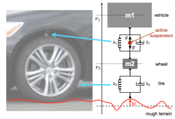
The active suspension control system essentially measures the displacement of the wheel and vehicle position relative to the “desired” ones, computes how to compensate for this error, and actuates with hydropneumatic or electromagnetic suspensions. The active element is represented by the circle producing a force F. Our overall goal is to automatically determine F to minimize the effects of the disturbance w (rough terrain) on the wheel and chassis displacement.
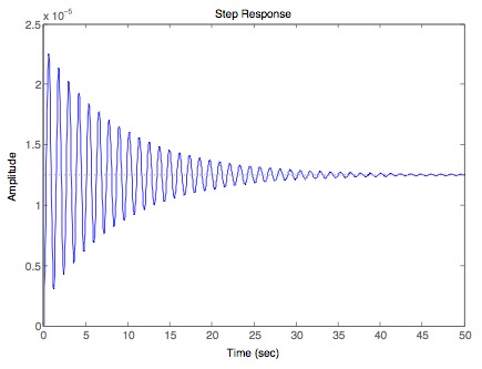
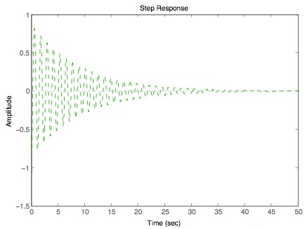
You will design and activate suspension system for a quarter car body and wheel assembly model using frequency domain design techniques. You will have to ensure passenger comfort by minimizing the amplitude and duration of oscillations in the car response to terrain disturbances.
| Subsystem | Masses [kg] | Spring constants [N/m] | Damping coefficients [M/m/s] |
|---|---|---|---|
| 1 | m1 = 2500 | k1 = 80,000 | b1 = 350 |
| 2 | m2 = 320 | k2 = 500,000 | b2 = 15,000 |
Mathematical Representation of the System and Stability Analysis
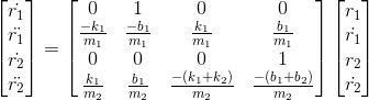
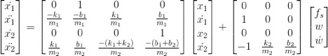
- State Space, ordinary differential equation model for the system

- Equilibria of the active suspension system assuming F and w are zero
- Stability Test
Using Matlab
Given: m1 = 2,500; m2 = 320; k1 = 80,000; k2 = 500,000; b1 = 350; b2 = 15,000;
A = [0 1 0 0; -k1/m1 -b1/m1 k1/m1 b1/m1; 0 0 0 1; k1/m2 b1/m2 -(k1+k2)/m2 -(b1+b2)/m2];
B = [0 0 0; 1 0 0; 0 0 0; -1 k2/m2 b2/m2];
eig(A)
ans =
	-23.9446 + 35.2083i
	-23.9446 - 35.2083i
	-0.1098 + 5.2504i
	-0.1098 - 5.2504i
All the real values of the resulting eigenvalues are negative. Therefore, it is factual to say the system is stable.
Laplace/Transfer Function Model for the System
In control theory, functions called transfer functions are commonly used to characterize the input-output relationships of components or systems that can be described by linear, time-invariant, differential equations. We begin by defining the transfer function and follow with a derivation of the transfer function of a differential equation system. The transfer function of a linear, time-invariant, differential equation system is defined as the ratio of the Laplace transform of the output (response function) to the laplace transform of the input (driving function) under the assumption that all initial conditions are zero.
- Take as the system output the difference between the two positions.
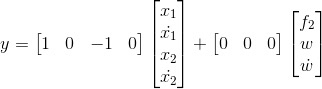
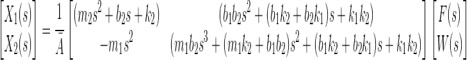
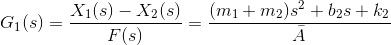
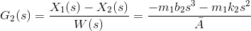
- Calculate the two transfer functions:
Between the active suspensor input F and the output y:
Between the disturbance input w and the output y:
[1]

[2]

[1] + [2]


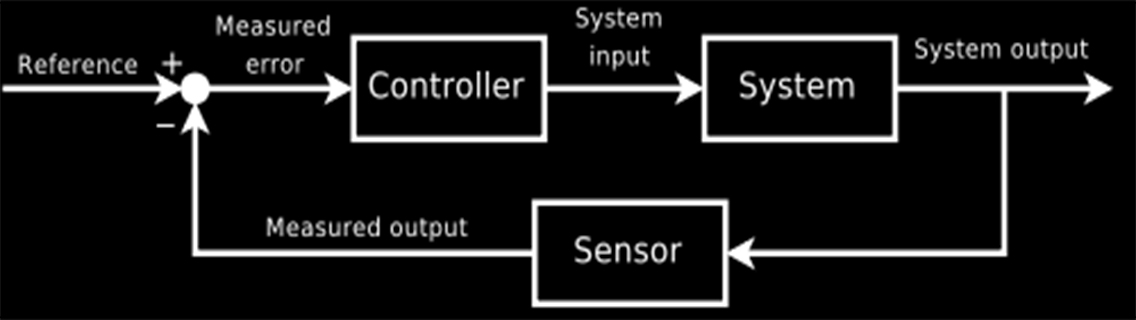
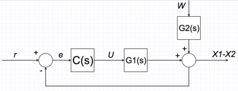
Introduction Feedback/Block Diagrams
A block diagram of a system is a pictorial representation of the functions performed by each component and of the flow of signals.
To draw a block diagram of a system, first write the equations that describe the dynamic behavior of each component. Then take the Laplace transforms of these equations, assuming zero initial conditions, and represent each Laplace-transformed equation individually in block form. Finally, assemble the elements into a complete block diagram.
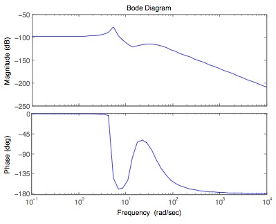
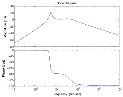
Bode Plots
A Bode diagram consists of two graphs: One is a plot of the logarithm of the magnitude of a sinusoidal transfer function; the other is a plot of the phase angle; both are plotted against the frequency on a logarithmic scale. The main advantage of using the Bode diagram is that multiplication of magnitudes can be converted into addition. A simple method for sketching an approximate log-magnitude curve is available. Note that the experimental determination of a transfer function can be made simple if frequency-response data are presented in the form of a Bode diagram.
Using Matlab
s = tf('s');
G1 = ((m1+m2)*s^2+b2*s+k2)/((m1*s^2+b1*s+k1)*(m2*s^2+(b1+b2)*s+(k1+k2))-(b1*s+k1)*(b1*s+k1));
G2 = (-m1*b2*s^3-m1*k2*s^2)/((m1*s^2+b1*s+k1)*(m2*s^2+(b1+b2)*s+(k1+k2))-(b1*s+k1)*(b1*s+k1));
w = logspace(-1,4);
bode(G1,w)
bode(G2,w)
Root Locus
By using the root-locus method the designer can predict the effects on the location of the closed-loop zeros. Therefore, it is desired that the designer have a good understanding of the method for generating the root loci of the closed-loop system, both by hand and by use of a computer software program. The root-locus method proves to be quite useful, since it indicates the manner in which the open-loop poles and zeros should be modified so that the response meets system performance specifications.
Using Matlab
rlocus(G1)
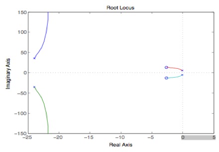
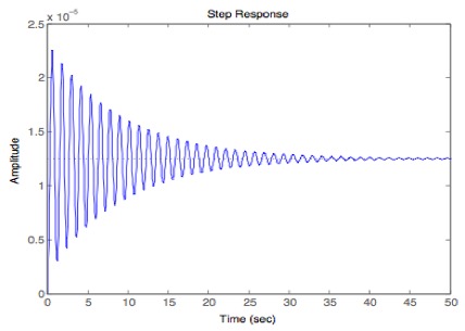
It is ideal to put a pair of poles and zeros near the imaginary axis to cancel out the poles and zeros currently there. After the poles and zeros are “cancelled” with the ones we added, it is best to put poles very far to the left to get a faster response, which will reach steady state faster. Having poles near the Imaginary axis will give a slow response, which makes the system oscillate a lot before reaching steady state.
Dr = -log(0.05)/sqrt(pi^2+log(0.05)^2)   %Dr = damping ratio
Dr = 0.6901
wn = 4.6/(1*Dr)   %wn = natural frequency
wn = 6.6656
Compensator Design
The compensator compensates for deficient performance of the original system.